Telemetry and Teleoperation of an mBot

TLDR Summary

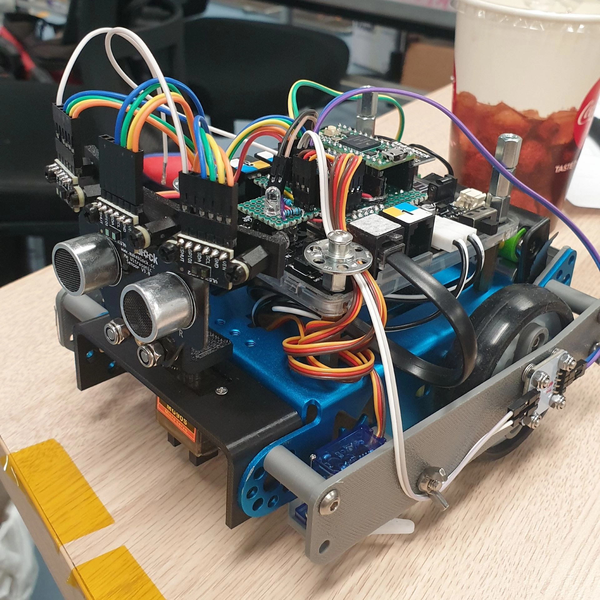
Added an encoder and IMU to an mBot to implement localisation, as well as used its onboard RF module to send its position to a separate computer. Video demo can be found in this section.

This project was part of the final assignment for EE2111A: Electrical Engineering Principles and Practice II, which is the second half of a two-part introductory module for Electrical Engineering.

The original task simply required us to program an mBot to move within a square area bounded by black lines while avoiding obstacles within it, simulating a robot vacuum. However, since the task did not require the robot to move in any specific pattern, the entire logic would have unironically been:

1
if (line_detected || obstacle_detected) turn_random_angle();
2
else move_straight();

Clearly that would have been a pointless exercise. This was when I realised that:

For all the localisation stuff I had done in the past, I never actually tried good ol’ wheel odometry
I had some magnetic encoders lying around from a previous experiment for FOC of a BLDC motor
I was bored out of my mind

Thus began my journey into adding telemetry to a literal children’s toy. The main considerations were to:

Use as much of the existing hardware as possible (NO SBC, NO ROS!)
Only use extra parts that I already owned or had access to.
Keep to the original theme of a vacuum robot; aim to emulate the older vacuum robots that used dead reckoning without LIDARs or cameras.
Ensure the robot is still able to complete the original requirements without any of the added components.

Overall Design

I have found that a useful purpose of these random mini-projects is to help keep my less utilised skills fresh, case in point, using MCAD software. This becomes especially important as the projects I do and roles I find myself in continue to dive into deeper levels of specialisation within Electrical Engineering.

Render of modified mBot in Fusion

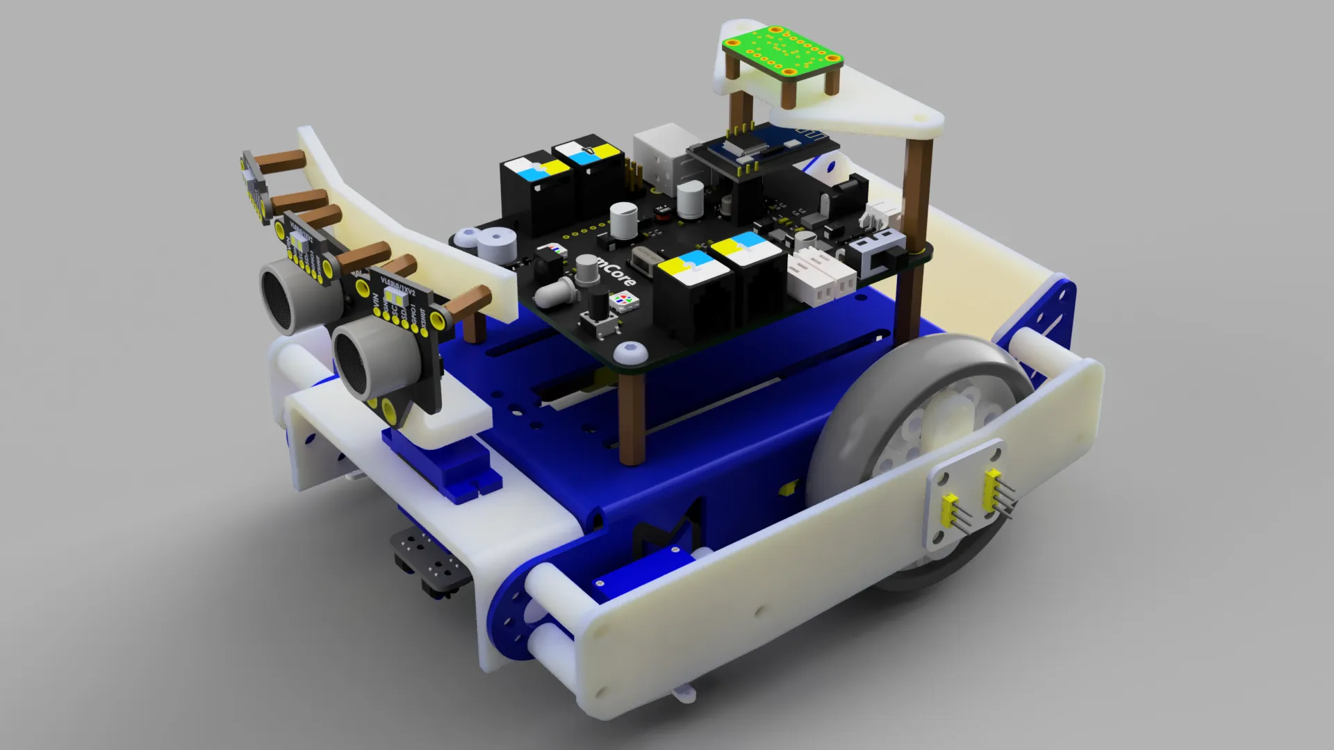
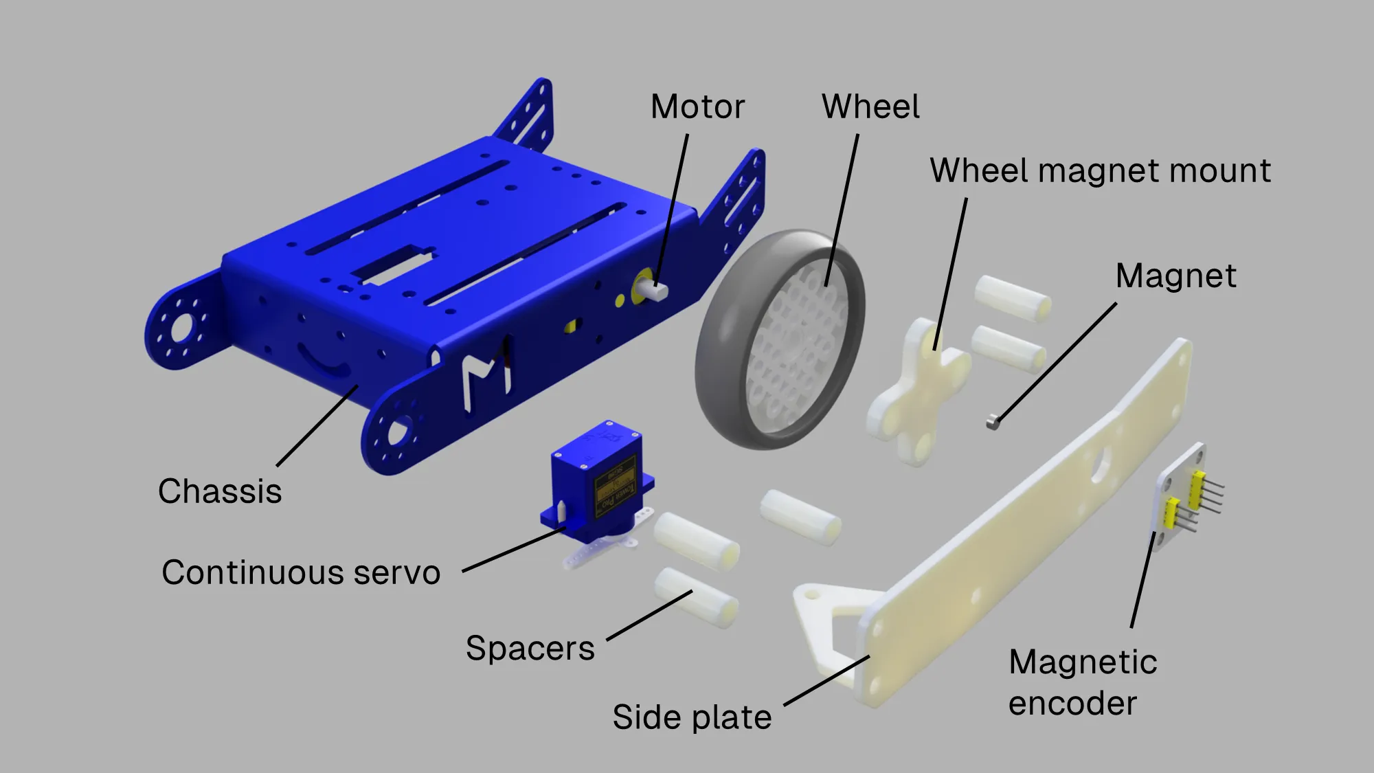
Mechanical

For the design, magnetic encoders were chosen partly due to its ease of installation compared to rotary or optical encoders. All that had to do be done was add a diametrically-magnetised magnet to the wheel and mount the encoder to an external plate. For the fun of it, continuous servos were also attached to these external plates at the front of the robot, simulating the side brushes of a robot vacuum.

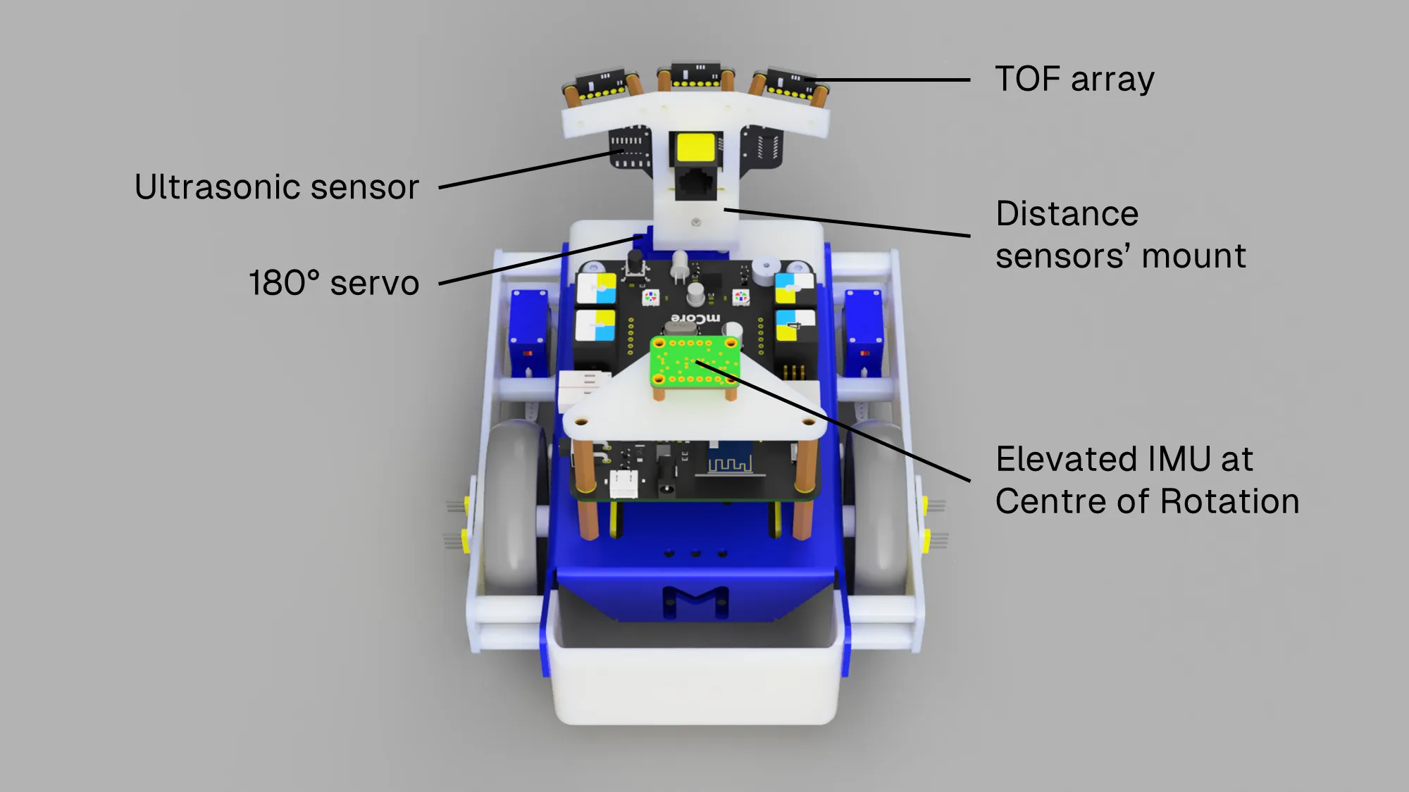
For other sensors, an array of TOF sensors were added and mounted onto a servo, which allowed it to rotate to face obstacles. The ultrasonic sensor was still included just to ensure compliance with the original requirements… 😒

Also, an IMU was placed at the centre of rotation (between the two drive wheels), physically elevated to minimise magnetic interference.

Exploded view of side of robot Back view of robot

Electrical

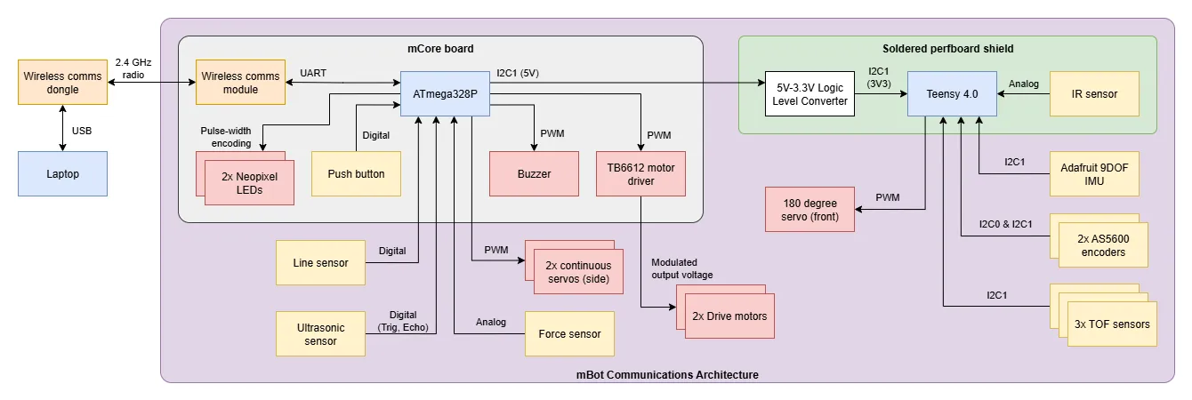
The mBot’s mCore control board uses the ATmega328P, which handled all my lower level processes, i.e. interfacing with the original mBot components e.g. line sensors, motor drivers, wireless communications, etc.

A Teensy 4.0 was used for interfacing with the added sensors like the IMU, TOFs, and encoders (necessary for encoders as they have fixed I2C address, so they needed to be on different I2C buses). The Teensy also handles the higher level processes like filtering and odometry.

Relevant information from the ATmega328P’s sensors were communicated over to the Teensy using I2C. The final calculated movement commands and state estimates were sent from the Teensy back to the ATmega328P for output/relaying to the computer.

All the added electronics were soldered onto a perfboard shield that neatly attached on top of the mCore board. The high-level communications architecture of the robot is illustrated below.

Electrical comms architecture

Magnetic Encoders

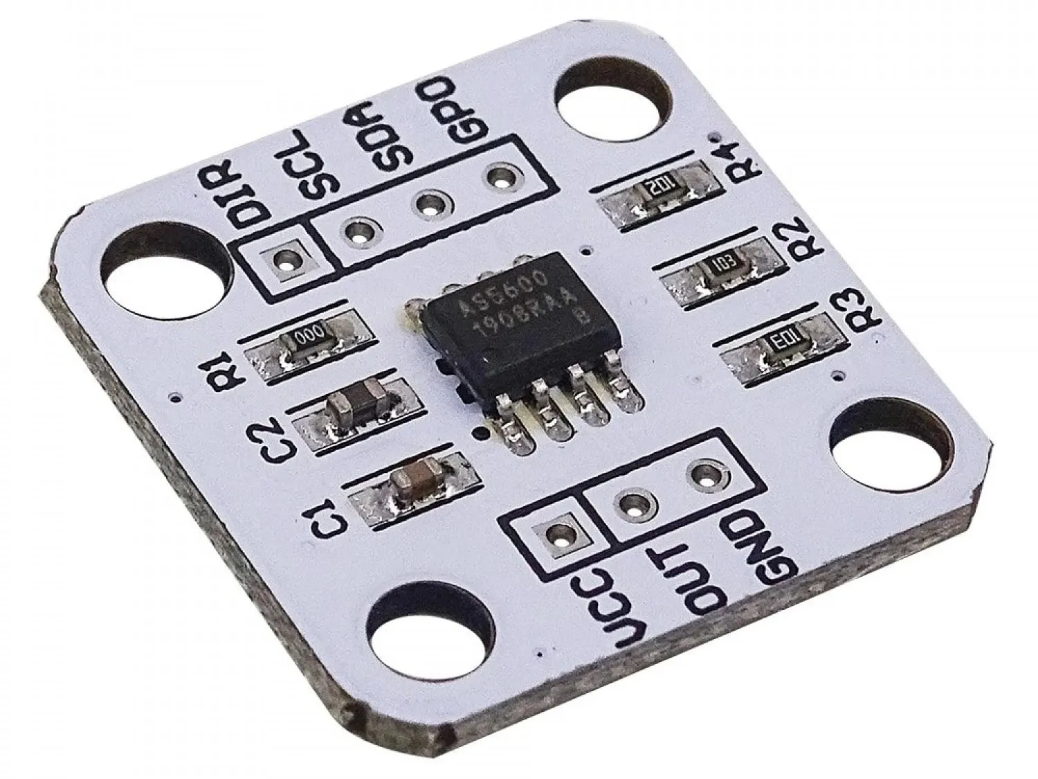
The magnetic encoders used were the common AS5600 breakout boards, which had a resolution of 4096 ticks per revolution. The absolute angle positions were communicated over I2C at a fixed polling rate of 1 kHz. (Image Source: TinyTronics)

AS5600 breakout board (mini-image)

Alignment Problems

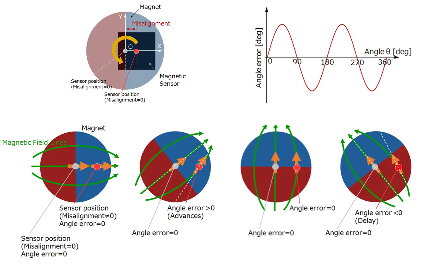
The main problem faced was aligning the encoder with the magnet properly. Internally, the encoder works by having hall-effect sensors that measure $B_{x}$ and $B_{y}$ , the magnetic field strength in the X and Y axes, where magnetic field angle $θ = arctan (B_{y} / B_{x})$ .

However, when the encoder is offset from the axis of rotation, an angular error is introduced which leads and lags periodically based on the phase angle, as illustrated below. (Image source: Asahi Kasei Microdevices)

Misaligned encoder angular error

These alignment errors were inevitable since the wheel was only supported at the motor shaft, causing a negative camber tilt, while the cheap breakout boards were not exactly known for having precise dimensions either. Hence, correction in software was required.

Fixing It in Post

The proper way to fix this would have probably involved some math-y signal processing mumbo jumbo but as an engineer after all, the easiest solution was simply… a lookup table!

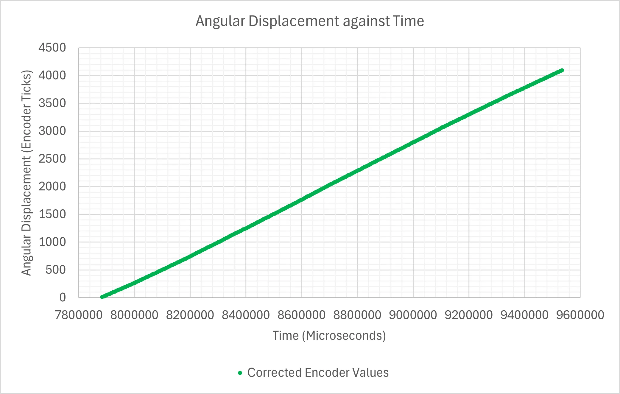
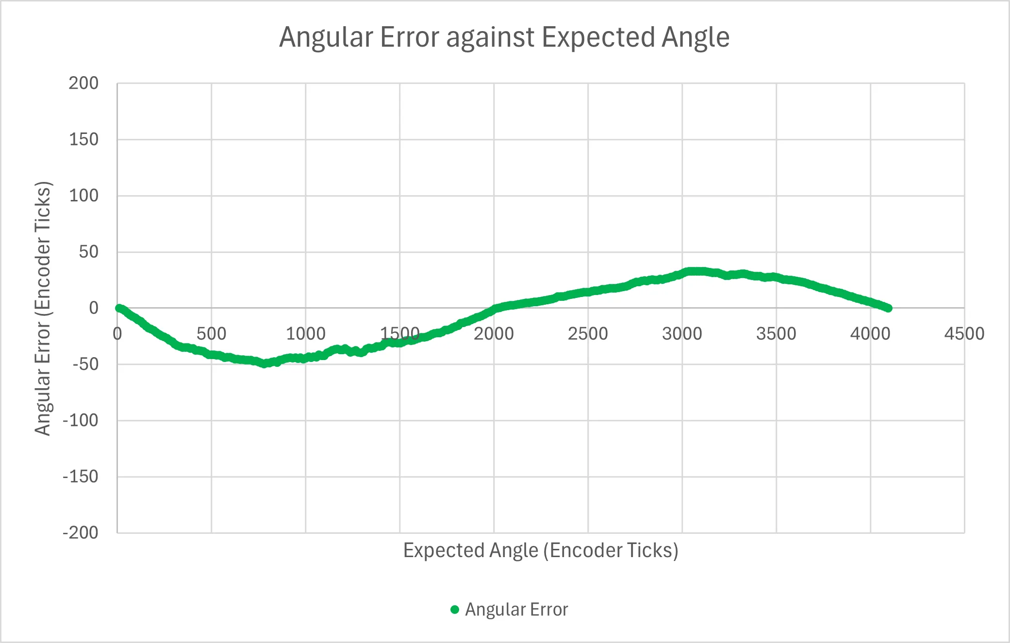
The graph on the left below shows the encoder’s measured readings while running the wheels at a constant speed (blue line). However, since the angular velocity is (relatively) constant, the expected readings should be linear, which can be interpolated from the readings (orange line). By plotting the error between the two values against the expected angle, we get the graph on the right showing the sinusoidal error as expected.

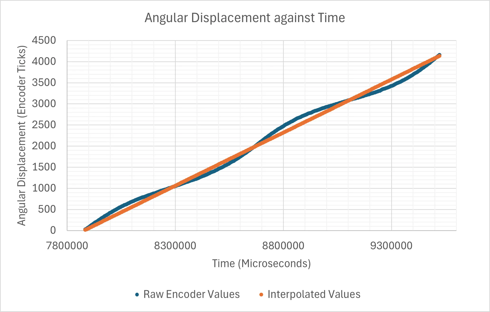
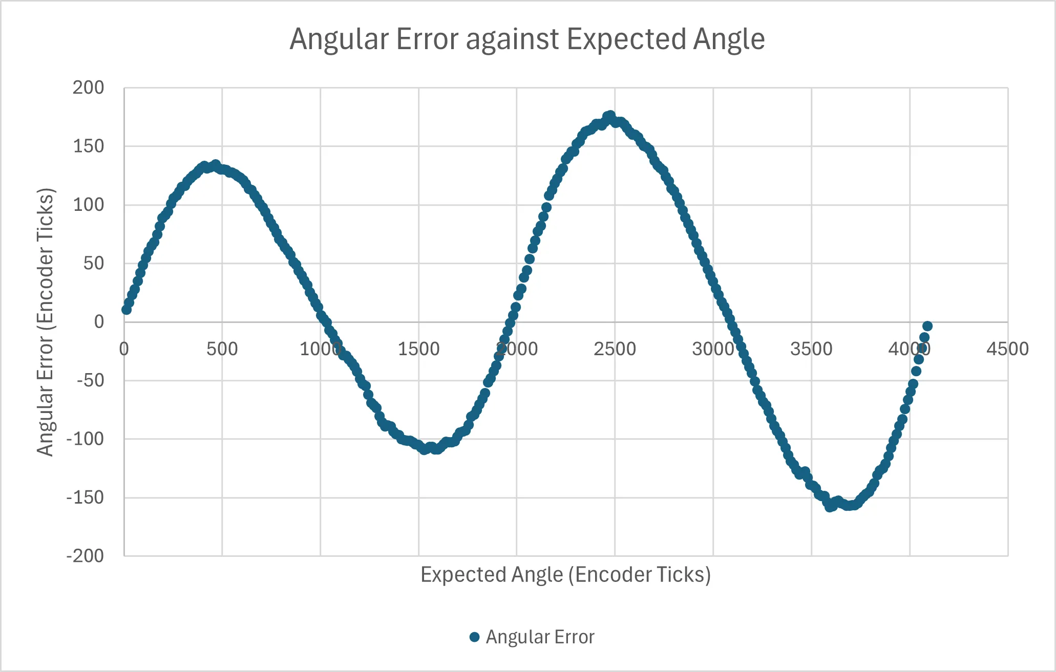
Raw encoder values vs interpolated values Angle error against expected angle

Using the interpolated values as references for a lookup table, every raw encoder reading could be mapped to its “correct” reading! In about 15 mins of fiddling on Excel and zero math, the encoder error was greatly reduced and now actually usable (some error still inevitably exists from the less-than-ideal structure of the mBot itself).

Corrected encoder values Minimised angle error against expected angle

PI Velocity Controller

With the alignment issue resolved, closed-loop control could now be added to the motors. Initially, I considered a cascaded controller with velocity control in the inner loop and position control in the outer loop. But, on second thought, almost all commands were going to be conditional on other sensors, e.g. move till line detected, or move based on IMU heading, so only velocity control was needed.

Hence, keeping things simple, a standard PI velocity controller was implemented. The derivative term is not necessary for velocity control as it has a tendency to add noise (velocity measurements with encoders are relatively noisy to begin with), and has minimal impact (a well-tuned PI controller will generally not produce rapid velocity changes to begin with).

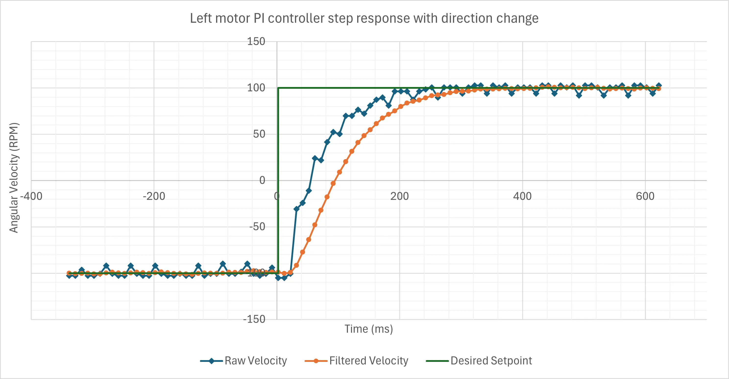
At each discrete time step, $k$ , the raw motor velocity, $V_{k_{r a w}}$ is approximated from the encoder angle’s change over time, $\frac{Δ θ}{Δ t}$ , followed by a first-order Butterworth filter to attenuate the high frequency noise and derive the filtered, smooth velocity, $V_{k_{f i lt ere d}}$ .

V_{k_{r a w}} = \frac{θ _{k} - θ _{k - 1}}{Δ t} V_{k_{f i lt ere d}} = \frac{V _{k_{r a w}} + V _{k - 1_{r a w}} + a \cdot V _{k - 1_{f i lt ere d}}}{b}

342
float left_angle_curr = lookup_convert(as5600_left.readAngle(), lookup_table_left, lookup_table_left_size);
343
float left_angle_dx = smallest_angle_between(left_angle_curr, left_angle_last, polarity=true);
344
float left_vel_raw_curr = left_angle_dx / ENCODER_DT;
345

346
//first-order butterworth, unit: ticks per sec
347
float left_vel_filtered = (left_vel_raw_curr + left_vel_raw_last + 6.916*left_vel_filtered)/8.916;
348

349
left_angle_last = left_angle_curr;
350
left_vel_raw_last = left_vel_raw_curr;

This filtered velocity becomes the process variable of the PI controller to produce the desired PWM value $u_{k}$ . The integral term, $I_{k}$ was set to freeze if $u_{k}$ reaches its limits so as to prevent integral windup.

e_{k} = V_{k_{d es i re d}} - V_{k_{f i lt ere d}} I_{k} = {I_{k - 1} + e_{k} I_{k - 1} if ∣ u_{k - 1} ∣ < 255 otherwise u_{k} = max (min (K_{p} \cdot e_{k} + K_{i} \cdot I_{k}, 255), - 255)

The final PI controller was tuned to be slightly over-damped with a 0.4s settling time, but that was acceptable for the smoother movement it produced.

PI controller tuned response

Side note: Doing all this reminded me of the “Move” blocks in Lego EV3-G, all the way back in primary school robotics. Life truly is nothing but a flat circle.

IMU + Wheel Odometry

The IMU used was the Adafruit LSM6DS3 + LIS3MDL 9-DOF IMU. The robot is assumed to always be on a flat surface, so I only had to be concerned with linear motion in the X-Y plane, and rotational motion in the Z-axis. From past experience with cheap IMU’s accelerometers, their high levels of noise made them unable to estimate planar motion accurately, so they were not incorporated into the sensor fusion process.

These assumptions/decisions meant fusion was only possible with the robot’s heading, which also made things much simpler! A standard Kalman filter on the magnetometer and gyroscope readings was implemented to estimate the robot’s heading (without needing tilt compensation either). This heading estimate was then fed into a second Kalman filter for fusion with the wheel odometry-based robot heading. Doing a cascaded filter also meant minimal changes needed to be made to the existing Kalman library.

For the actual mathematical details, the Kalman Filter library’s accompanying blog post explains it well, but a brief summary of my use case is as follows.

Gyro + Magnetometer Kalman Filter

The first Kalman filter (for gyroscope and magnetometer) was kept identical to the original library. The state vector at each timestep $k$ contains the robot’s heading $θ$ and the gyroscope’s bias $\dot{θ}_{b}$ :

x_{k} = [θ \dot{θ}_{b}]_{k}

The state of the system is modelled by:

x_{k} = F x_{k - 1} + B \dot{θ}_{k} + w_{k} F = [10 - Δ t 1], B = [Δ t 0]

where $F$ is the state transition matrix, $B$ is the control input matrix, $\dot{θ}_{k}$ is the gyroscope’s Z-axis angular velocity reading, and $w_{k}$ is the process noise. This is simply stating that the predicted angle in a new time step is a sum of the previous angle (minus the bias), the change in angle over the time step (assumes constant angular velocity during the time step, which is valid for high update rates since the angle change is small), plus random Gaussian noise. The bias remains unchanged as it cannot be calculated directly from the gyroscope readings.

For the measurement vector, it is modelled by:

z_{k} = H x_{k} + v_{k} H = [10]

where $H$ is the observation matrix, $v_{k}$ is the measurement noise. The only measurement is the magnetometer’s calculated heading, which is simply $arctan (B_{y} / B_{x})$ (flat ground assumed so no tilt compensation needed).

Wheel Odometry

For the wheel odometry, the robot’s position and heading can be estimated relatively accurately from the wheel encoders through basic Euler integration since the time difference $Δ t$ between each time step $k$ is small and fixed. The robot’s low top speed and acceleration also meant that wheel slip would be negligible. Given the wheelbase distance $b$ and the distance travelled by the left and right wheel, $Δ s_{L}$ and $Δ s_{R}$ respectively,

x_{k} = x_{k} y_{k} θ_{k} Linear displacement, Δ s_{k} = \frac{Δ s _{L_{k}} + Δ s _{R_{k}}}{2} Angular displacement, Δ θ_{k} = \frac{Δ s _{L_{k}} - Δ s _{R_{k}}}{b} x_{k + 1} = x_{k} + Δ s_{k} \cdot cos (θ_{k} + \frac{Δ θ _{k + 1}}{2}) y_{k} + Δ s_{k} \cdot sin (θ_{k} + \frac{Δ θ _{k + 1}}{2}) θ_{k} + Δ θ_{k + 1}

Fusing Heading Estimates

For combining heading estimates with a second Kalman filter, I used the angular displacement from the wheel odometry in the prediction step, while the fused IMU heading was used in the measurement step. No bias was needed in the state vector as the encoder readings did not suffer from drift.

The more proper way to do this would have probably been to use an Extended Kalman Filter and combine the state and measurement vectors so that position and heading can be calculated in a single step, but this method was the quickest way (adapt existing library with minimal edits) while being simple to tune. Regardless, I did not have the time to explore further anyway, so we move on!

2.4 GHz Wireless Communications

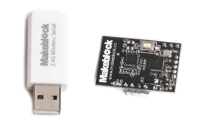
The mBot comes with a 2.4 GHz wireless serial module connected to the onboard ATmega’s UART lines,and a USB dongle which is meant to allow for wireless program uploads. Image Source: Makeblock

2.4 GHz wireless module (mini-image)

Receiving Data

I wanted to piggyback off of this module to send telemetry data, but there was somehow absolutely zero information about this module online. So, starting from the fact that the dongle was a HID device, I tried to directly dump its raw data to see what it was sending/receiving.

In this world nothing can be said to be certain, except death and taxes… and that a Python library already exists for the problem you’re trying to solve.

~ Benjamin Franklin, probably

Using hid, a Python binding for the hidapi library, I could scan all the connected HID devices to retrieve the USB dongle’s vendor ID (0x0416) and product ID (0xFFFF).

Dumping its received data, it turns out the dongle returns a byte array of length 30 on every read call. If no data was being sent, then the whole array would simply be made up of NULL characters. If there was data, then the received bytes would be scattered somewhere in the byte array, and sometimes annoyingly split across two messages.

To combat that, messages from the mBot were sent as comma delimited strings with a vertical bar ’|’ as an end delimiter. On the receiving end, incoming bytes were stored in a buffer which only got parsed into floats when the end delimiter is read.

91
def update_state_vector(state_vector:list, msg_buf:str):
92
    '''
93
    Updates state vector if complete serial message is received. Returns 1 for change, 0 for no change.
94
    msg_buf: keep track of bytes from past messages
95
    state_vector format: [pos_x (m), pos_y (m), angle (rad), line_detected (0=none, 1=left, 2=right, 3=both)]
96
    '''
97
    msg = hid.Device(HID_VID, HID_PID).read(31)  #30 is the usual msg bytes length
98
    for byte in msg:
99
        if byte == 0x7C:    #0x7C = '|' = end delimiter
100
            clean_msg = ''.join(msg_buf)
101
            msg_buf[:] = []
102
            break
103
        elif byte > 0x20:  # ignore control characters \\0,\\r,\\n
104
            msg_buf.append(chr(byte))
105

106
    try:
107
        temp_vector = [float(i) for i in clean_msg.split(',')]
108
        if (len(temp_vector) == 4):  # end delimiter sometimes get dropped so two messages merges
109
            state_vector[:] = temp_vector
110
            return 1
111
        else:
112
            return 0
113
    except: # catch all for incomplete messages or other garbled chars
114
        return 0

The final status update rate was set to around 20 Hz, which was a good balance between the realtime-ish updates for my GUI, and maintaining a high message success rate at longer distances. Some characters did still occasionally get dropped, but the failure rate was low enough that I could just ignore the erroneous message and wait till the next update.

Sending Data

With a little trial and error, it was found that messages sent from the computer to the mBot had to be null-terminated strings, and that the first 2 bytes of the string were always dropped (perhaps originally used as control characters).

124
hid.Device(HID_VID, HID_PID).write('001\0'.encode())  #received as '1' by mBot

The messages implemented were movement commands, turning the front servos on/off, and changing the Neopixel LEDs’ colour.

GUI

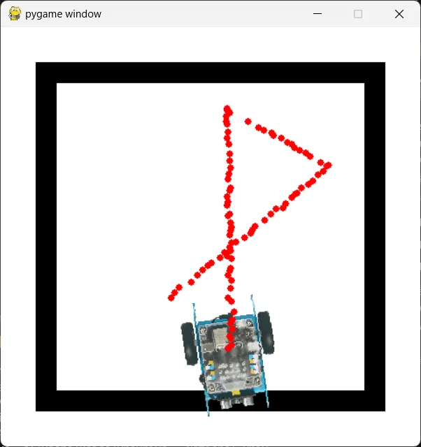
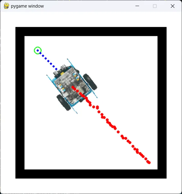
Finally, with the robot’s state, all that was left was to visualise it! While I used the Arcade library when building a robot simulator in the past due to its built-in physics engine, I stuck to the basic Pygame library this time since all I needed was to move a sprite around the screen.

The GUI simply reads the state vector received, converts the distance from metres to pixels (with the square border as a size reference), and updates the mBot sprite’s position and orientation on screen. When set to the teleoperation mode, key presses were recorded, allowing the user to move the robot with the arrow keys, or control its other peripherals. Alternatively, by clicking on the screen, the target position is converted to relative polar coordinates and sent to the robot, where it will turn and move to the target.

Screenshot of GUI with robot moving randomly

Of course, more could have been added, especially showing of obstacle positions, but by this point I had (1) spent way too much time on what was meant to be a throwaway project, and (2) was coding this up literally minutes before the evaluation, so… it is what it is.

Video Demo

Sadly, I have a habit of not regularly taking photos or videos of things I’ve built (which I hope having this website helps to fix). The best I could find is a short demo where the robot is teleoperated from the laptop’s arrow keys and doing random movement, all while having its position visualised on screen.

Areas For Improvement

As with most projects born out of personal interest, the more I did, the deeper the rabbit hole got, and the number of possible things to try out kept increasing. Considering I only had 2 weeks while juggling more important projects like EE2028 and other modules, many of these interesting ideas were not explored.

Nonetheless, I shall list some of them with a rough approach to how they would have been implemented, perhaps as “inspiration” for a future me.

Obstacle tracking
- The TOFs’ were positioned in a slight arc such that their ROIs overlapped slightly. <image>
- So if an obstacle was in front and to the left of the robot, the left TOF would detect that obstacle. The servo of the TOF array could then turn counterclockwise until the obstacle is no longer seen by the left TOF, which means it is now centred relative to the middle TOF.
- The servo’s angle thus provides a coarse estimate of the obstacle’s angle relative to the robot, which combined with the TOF’s measured distance provides relative polar coordinates of the tracked obstacle.
- Since the servo can spin up to 90 degrees in both directions, this opens up possibilities for wall-tracking, orbiting around obstacles, or avoiding moving obstacles.
- A primitive version of tracking was implemented by incrementing/decrementing the servo angle by a small, fixed amount when an obstacle is detected by the left/right TOF, but I never got to do more with it.
Using line boundaries as localisation landmarks
- Assuming the boundary dimensions are known beforehand, every time the robot detects a line, it can be used as a reference point of 100% certainty.
- This is similar to my localisation algorithm in RoboCup, but here, with only 2 light sensors and a smaller area, more thought would have to be put into how to differentiate between the vertical and horizontal boundaries.
EKF sensor fusion
- As mentioned in the odometry section, an Extended Kalman Filter with an expanded state vector that includes velocities or a full 6-DOF attitude estimation could allow for more accurate localisation.
- More rigorous exploration of the accelerometer could be done to incorporate it for sensor fusion and potentially compensate for wheel slip.

Concluding Thoughts

To be honest, there were much better uses of the time spent on this project, ~~like actually studying for my linear algebra module~~. Nevertheless, it has always been these kind of dumb side projects that has helped keep me sane (yes, doing more work to avoid doing other work) (so maybe not that sane after all).

For what it’s worth, it was while dismantling this robot that I realised how all the things I have built in the past (and will continue building both in university and in work), would similarly disappear if no documentation was kept. That was when I decided to make this website, not only as a portfolio, but also as a memory bank for random things I have learnt.

Here’s to many more hours wasted doing many more dumb things.

← Back to projects

Contents