Underwater Acoustic Positioning System
TLDR Summary
Built an acoustic positioning system for an AUV, with initial success from testing with collected data. Also oversaw the creation of the full electrical stack of the AUV, ensuring ease of maintenance.
As part of the training programme for Bumblebee, first-year prospects are tasked to build an Autonomous Underwater Vehicle (AUV) from scratch to participate in the Singapore AUV Challenge (SAUVC).
I was in the Electrical team, specifically doing Acoustics. One of the challenges in SAUVC consisted of a row of buckets on the pool floor where one of them contained a 45 kHz pinger, and the AUV had to locate and drop a ball into it.
Hence, I built the AUV’s acoustic positioning system to determine the azimuth and elevation of the underwater pinger. Although the final robot run did not tackle this mission due to other issues, bench tests and testing from collected data showed the system was able to locate the pinger to within ~1 degree of accuracy. Hence, I found this to still be worthy of documentation and the sections below detail the development of the acoustic system’s hardware and software.
As the co-lead of the Electrical team, I also oversaw the design of the overall electronics stack of the AUV, so the broad considerations for the overall electronics stack will be covered in the last section.
Mechanical Design
The hydrophone models used were inherited from the previous batches, which were the Sparton PHOD-1. These were omni-directional hydrophones with an integrated pre-amplifier.
Hydrophone Array
On determining the shape of the hydrophone array, it is self-evident that the number of dimensions in the array’s shape is related to the number of angular dimensions that can be resolved without ambiguity.
For an array of 2 or more co-linear hydrophones (i.e. 1D array), it can reliably measure time differences within a flat semi-circular plane. Only azimuth can be determined since the signal must be projected onto a plane that intersects with the array axis, at a fixed elevation angle. There is also “front-back” ambiguity since the readings coming from a source that is perpendicularly mirrored across the array’s axis cannot be differentiated with the original source, which is demonstrated in the figure below with the orange and green sources.
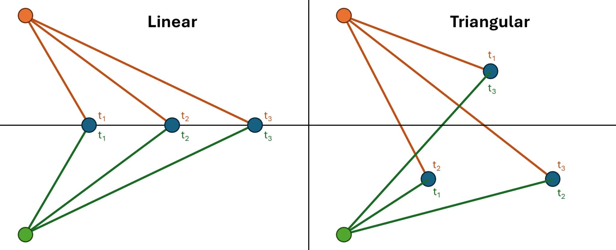
A triangular array (or any 2D shaped array), helps resolve the ambiguity by adding a 2nd dimension, and can reliably measure time differences within a hemispherical range. However, as the diagram below shows, while azimuth and elevation can be determined, there remains a “top-bottom” ambiguity since the readings coming from sources that are directly mirrored across the hydrophone array’s plane will result in the same measured time differences.
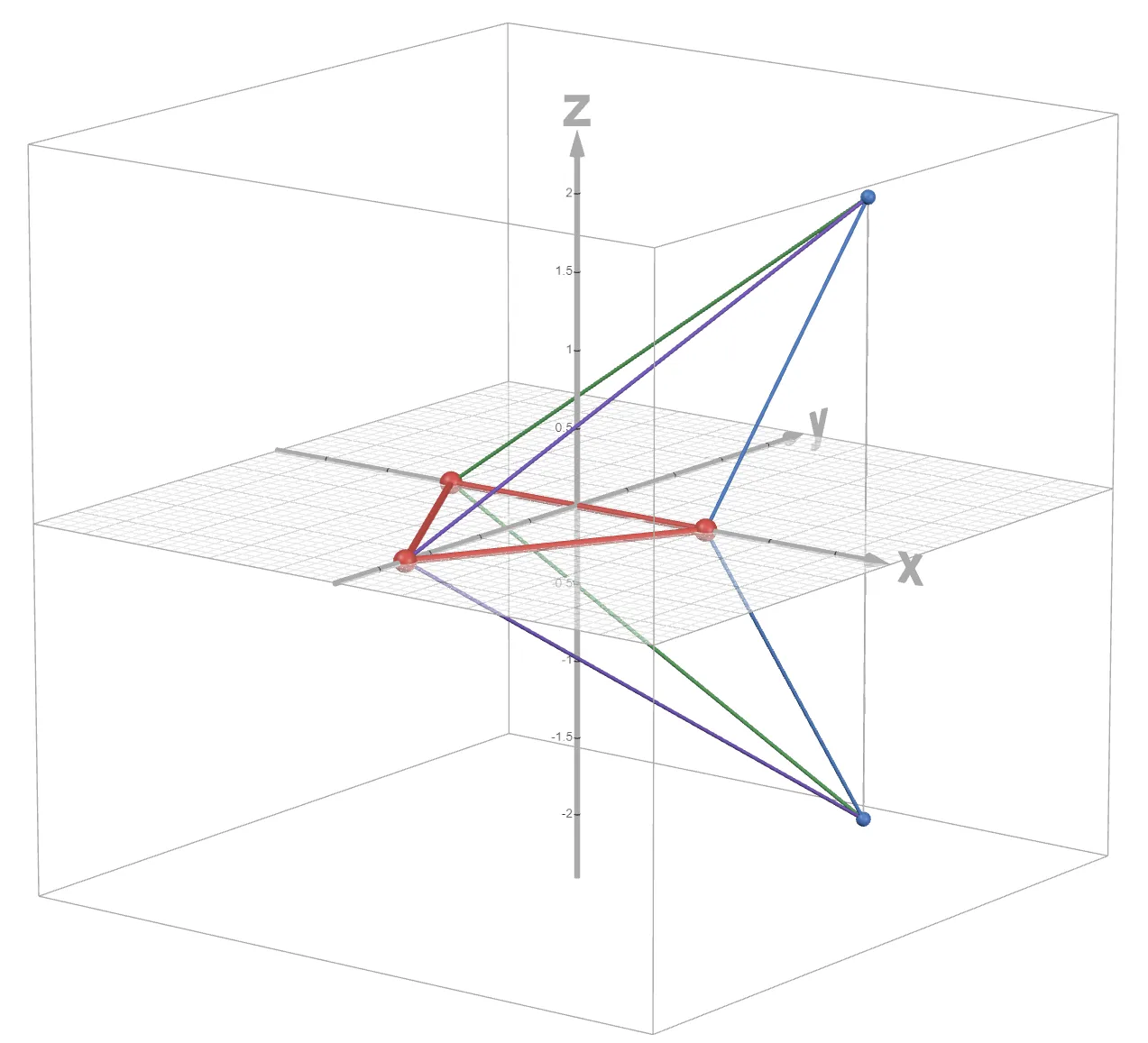
The usual way to fix this would be adding a fourth hydrophone in a tetrahedral arrangement, thus achieving the full 3D array. However, for my specific use case, since the pinger is located on the bottom of the pool floor, I could assume the pinger is always below the AUV, hence the triangular arrangement was sufficient. It would also have been much more complicated to design a tetrahedral mount, especially since the hydrophones were large.
Hydrophone Spacing
Another area of concern is the distance between hydrophones. As the polling rate is not very high (only about 3x above the pinger frequency), using time difference of arrival is likely too inaccurate. Hence, I relied on phase differences instead. This meant the spacing between each hydrophone should be less than 1 signal wavelength to prevent aliasing (grating lobes). Assuming speed of sound in water and pinger frequency , the signal’s wavelength .
However, the diameter of the hydrophone itself is , which meant it was not really feasible to go below the one wavelength limit. Also, these old hydrophones had to be used due to budgetary constraints, so there was no other way but to come up with software workarounds for the aliasing issues.
The final arrangement of the hydrophone was an equilateral triangle with side lengths of .
Hydrophone Placement
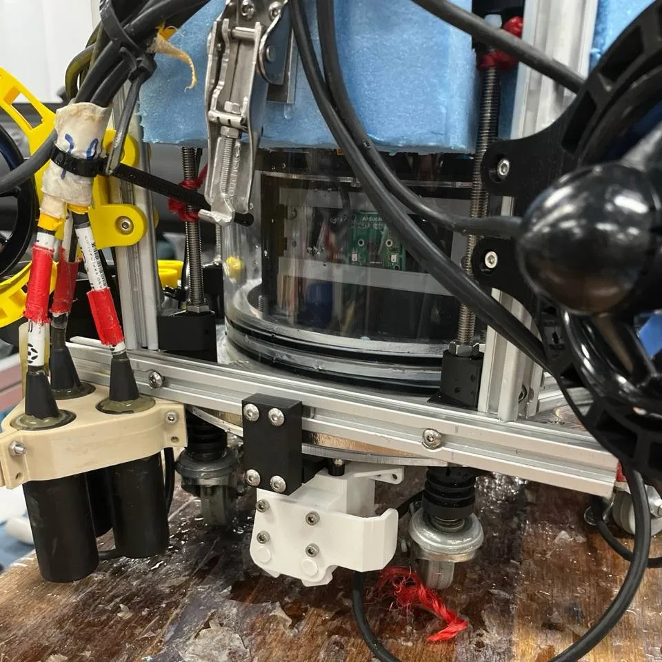
Since the AUV would mostly be facing forward, the hydrophone array was mounted on the front of the vehicle, offset to the right to provide a clear camera view, as shown in the picture below.
Electrical
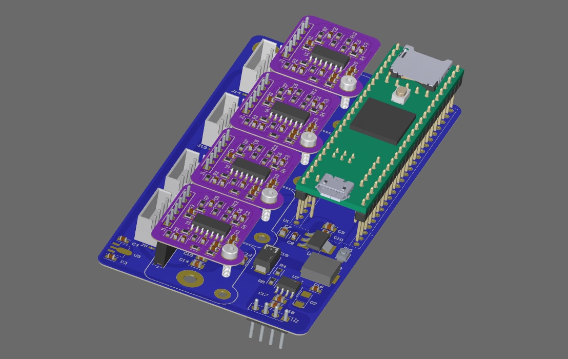
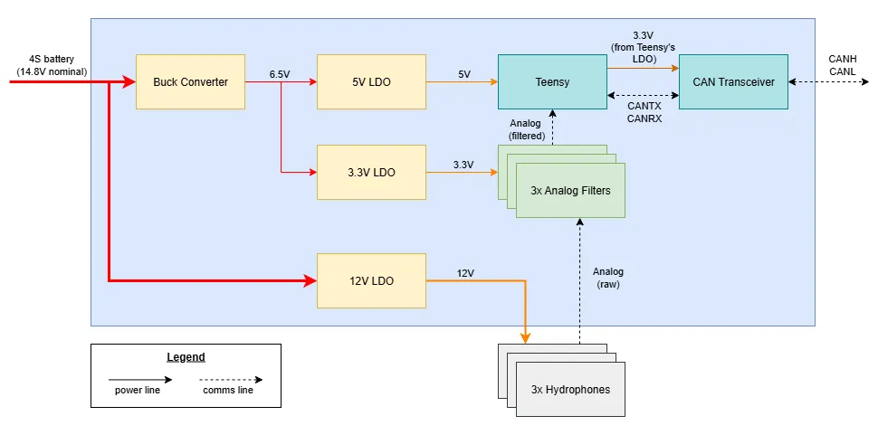
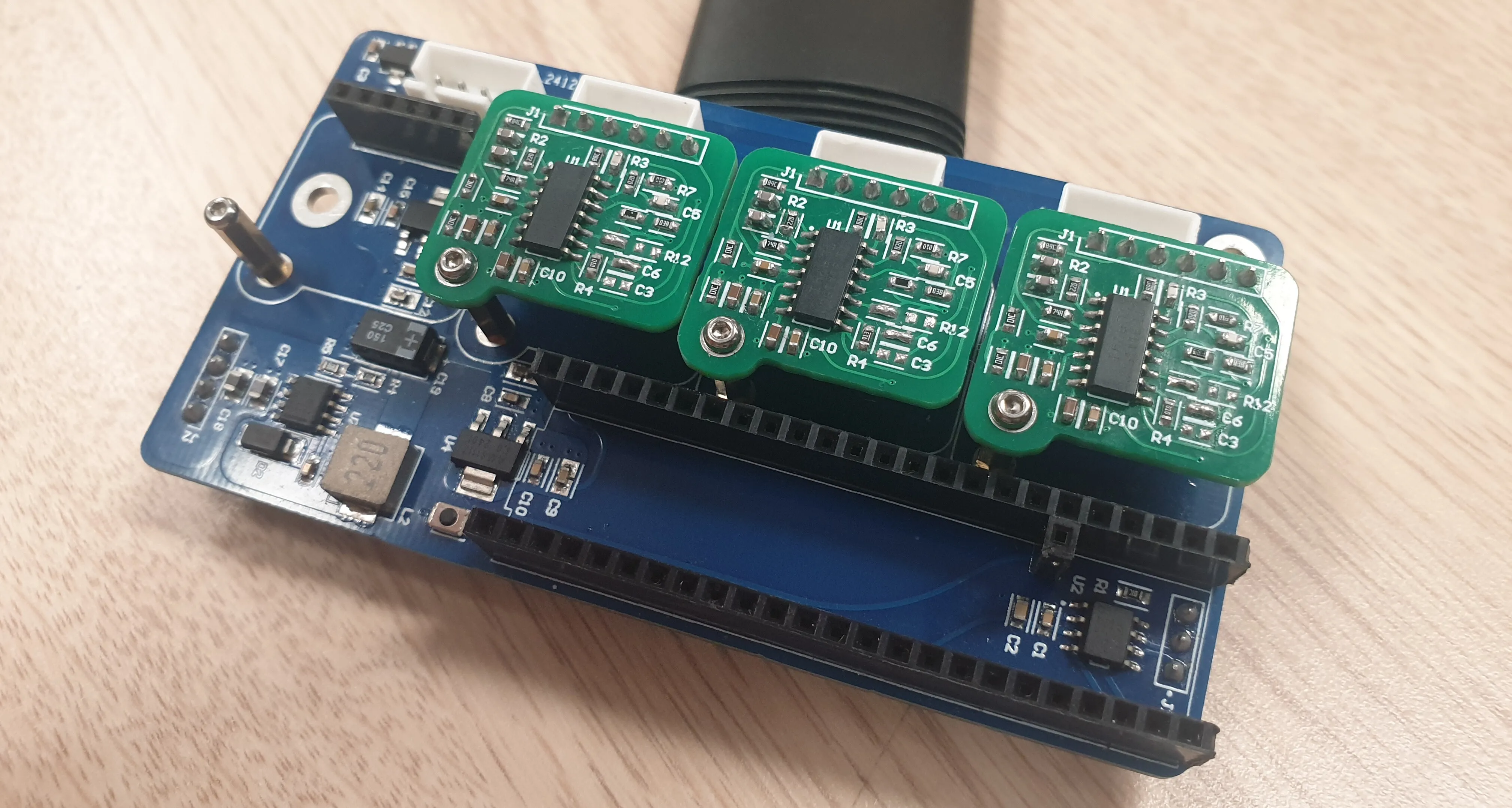
The overall electrical architecture of the acoustic system is shown below. The three hydrophones’ measurements fed into their individual analog filters, which were then sampled by the two onboard ADCs on the Teensy 4.1. Each analog filter PCB was its own separate board that sat above the acoustics motherboard PCB using header pins.
Analog Filter PCBs
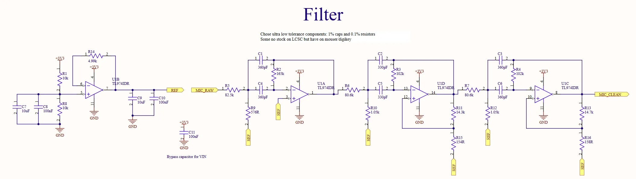
As there was only one pinger frequency at 45 kHz, a band-pass filter was created to sharply filter out signals from all other frequencies above and below this central frequency.
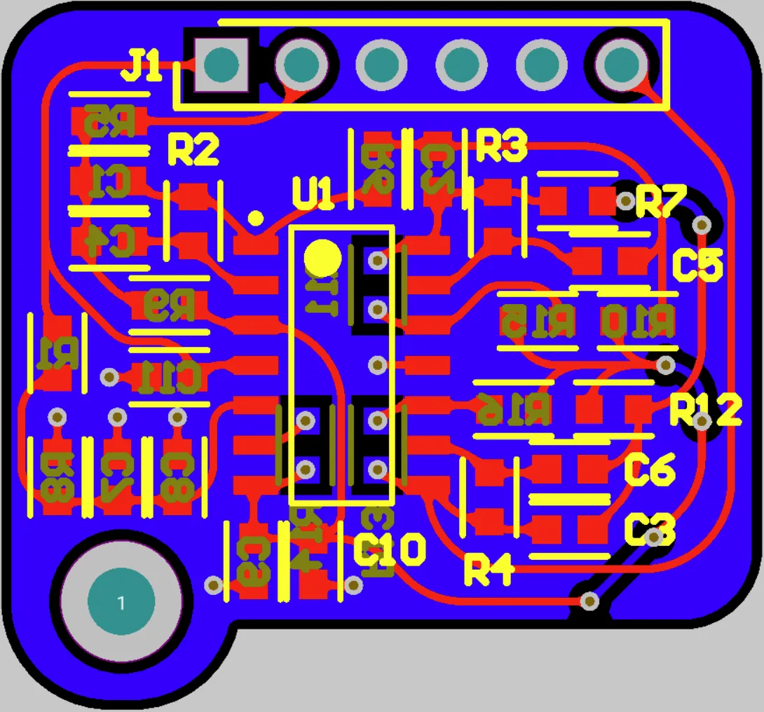
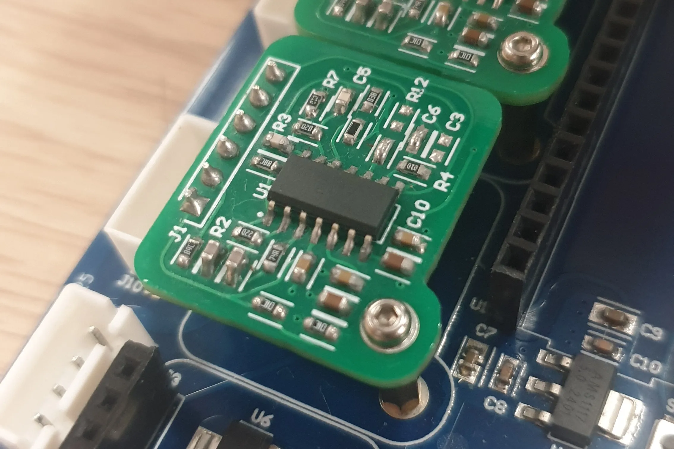
Using the Analog Devices’ Filter Wizard, a sixth-order Bessel filter was created with a relatively narrow 4khz passband. Also, given that it was not a complex board, I took the opportunity to have some fun by making all the traces smooth curves, which gave it that vintage/homemade PCB aesthetic.
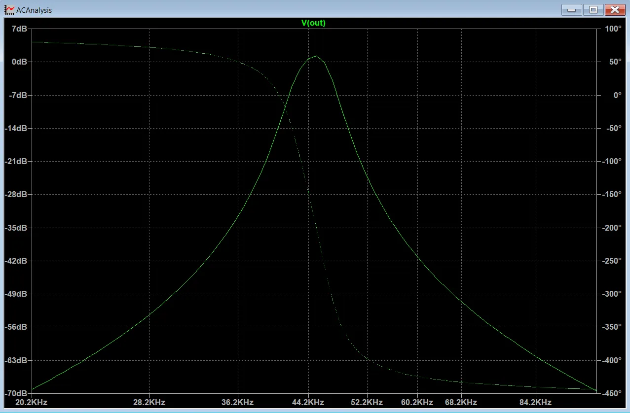
While this initially worked, upon assembling more boards, I found that the performance was inconsistent between different boards, e.g. different phase shifts, different attenuation levels.
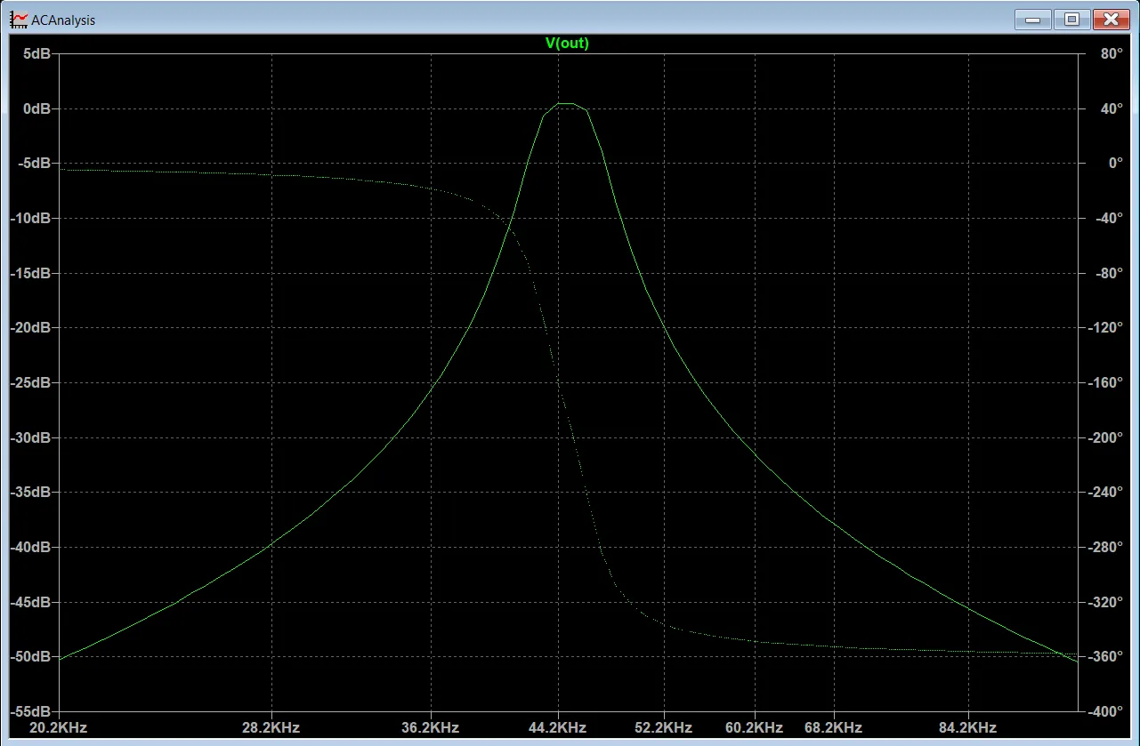
To cut a very long story of debugging, hair-pulling, and many rounds of LTspice simulations short, my conclusion was that the final filter stage was highly sensitive to parasitics, since all output signals from the prior 2 stages were perfectly fine. To solve this, I converted the filter into a 2-stage filter by converting the first stage into a unity gain inverting buffer, then changing as little of the remaining passive components as possible to get a similar frequency response. The final filter essentially had the same frequency response as the initial filter, but with a slightly narrower passband. However, since we can be quite confident that the pinger will remain strictly within 45 kHz, this fix was good enough.
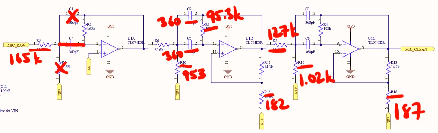
Till now, I am still not fully convinced the component sensitivities could cause such a large difference in the output, but empirical testing did show all the boards to have the same output at the second stage and only differing wildly from the third stage onwards. Black magic stuff.
The video below shows the filter PCB hooked up to a signal generator and oscilloscope, successfully attenuating signals below and above 45 kHz.
Motherboard PCB
The main purpose of the motherboard PCB was to provide clean power supplies 12V, 5V & 3.3V, as well as house the main microcontroller, a Teensy 4.1.
The Teensy 4.1 was chosen as it had an integrated, easy-to-use package. It had relatively fast ADCs, a built-in SD card slot for datalogging, and its high-speed processor could easily handle all the computational requirements.
For power, the raw battery power (4S LiPo, 16.8V max) was directly fed into an LDO regulator for a clean 12V source for the hydrophones. For the lower voltages, the battery power was first fed into a standard TPS5430 buck converter to lower the voltage down to 6.5V, followed by an LDO regulator to 5V and 3.3V, which partially helped with the ripple rejection too.
The motherboard PCB provides up to 4 channels with detachable analog filters, although the final configuration only required 3 hydrophones.
Software
As I only had to find a single source at a single frequency, I derived the approach below through first principles. In short, the algorithm did the following:
- Poll the 3 analog channels, then record their voltages and time of recording into circular buffers of size .
- For every pre-set samples read, perform DFT on the earliest readings.
- If a spike at 45 kHz is detected, then a ping has been detected and sinusoidal regression is performed on the latest readings to get their phase shifts.
- Comparing the phase differences between 2 pairs of hydrophones, get the range of possible azimuth and elevation angles.
- Resolve the final vector by using the signal arrival order or fusing with other sensor data.
Getting Signal Phases
The first step was to poll the analog channels as fast as possible. The Teensy 4.1 has 2 onboard ADCs which have a max sampling rate of 1 MSps (megasamples per sec) by using DMA and continuous conversion. However, as 3 channels needed to be polled, the ADCs had to switch between the analog channels, which required some stabilisation time after the channel is changed. Hence, after including all the other computational requirements needed for calculating pinger location, the final sampling rate was only around 125 kSps per channel. In hindsight, a separate high speed ADC should have been used for each channel. This would have allowed for more accurate time difference measurements, which would have avoided the spatial aliasing issues faced downstream.
Regardless, the final implementation used a hardware timer that triggered at 3 times the frequency of the ADC sampling rate. Upon each trigger, one of the ADCs is read and then switched to the next channel, while a conversion is started on the other ADC. When the ADC conversion is complete, the ADC interrupt callback will write the converted ADC reading and the current clock cycle count into separate circular buffers of length 128.
This allowed each of the 3 channels to be polled in a fast, rolling basis while providing sufficient settling time before each A/D conversion.
The next step was to detect a ping by performing DFT every few readings on the earliest 64 values in the circular buffer. However, since I am only concerned with the pinger’s frequency, I only need to perform the DFT summation at 45 kHz, not the entire frequency spectrum. Hence, the values samples, , (sampling period) were fed into the DFT equation below:
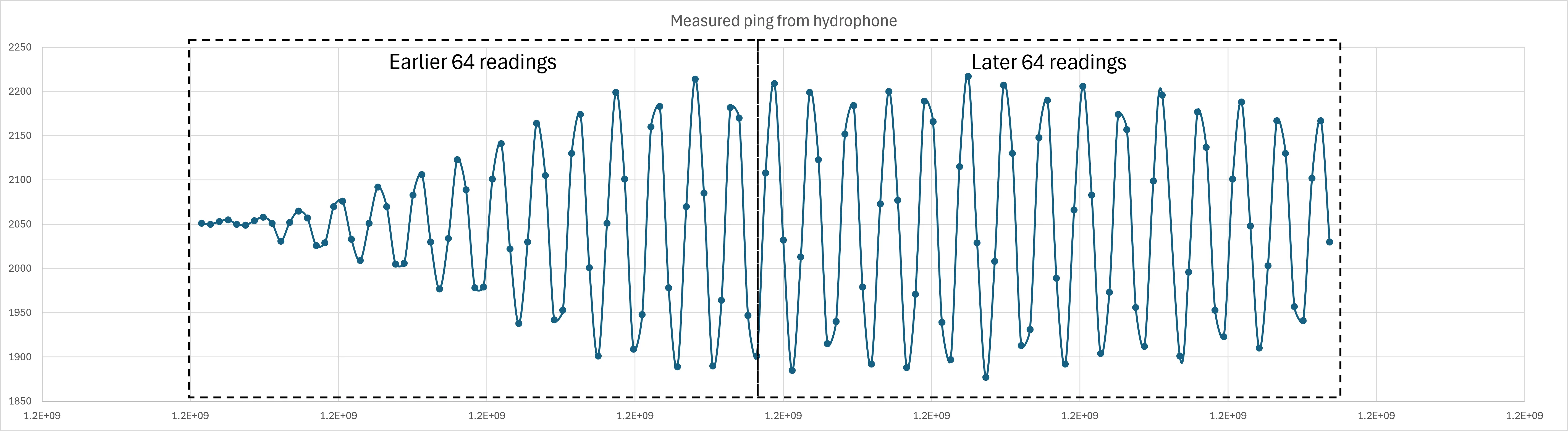
When exceeds the respective thresholds of each of the 3 hydrophones, then a ping is considered detected. Sinusoidal regression is then performed on the latest 64 values in the circular buffer to reconstruct the pinger signal. The preceding 64 values used for ping detection will still have a growing amplitude as shown in the figure below. Hence, regression is performed on the later part of the signal when readings have stabilised.
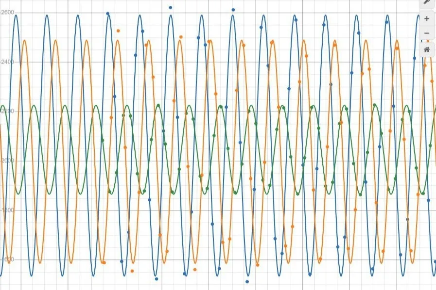
The lines in the graph below merely connect from one point to another with some smoothing for easier visualisation of the signal. It is NOT an actual sinusoidal regression line.
Sinusoidal regression is done by linearising the general sinusoidal equation , where since we can assume the signal amplitude is centred at 0.
where and are constants to be determined in a bivariate linear regression of and . Using the standard formulas for a bivariate linear regression, the constants are given by,
With the constants derived, the phase offset (the value in the original sinusoidal equation) can be found as such:
Direction Finding
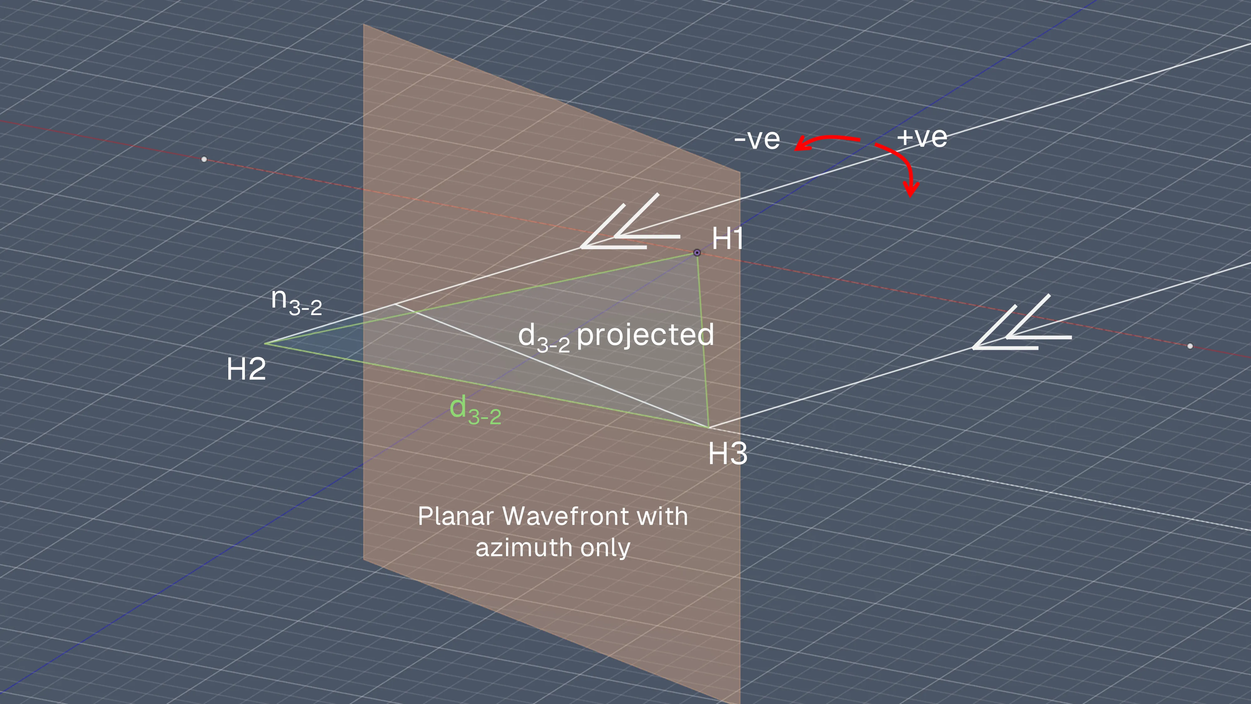
I first started with a simpler problem: deriving the phase difference given an azimuth and elevation angle. I chose the following conventions:
- H1 is the hydrophone in front, H2 is on the rear left, H3 is on the rear right.
- Clockwise rotations from the forward direction is positive azimuth, anti-clockwise rotations are negative azimuth.
- Elevation angle is relative to hydrophone array plane, so since all sources are below this plane, all elevation angles are negative.
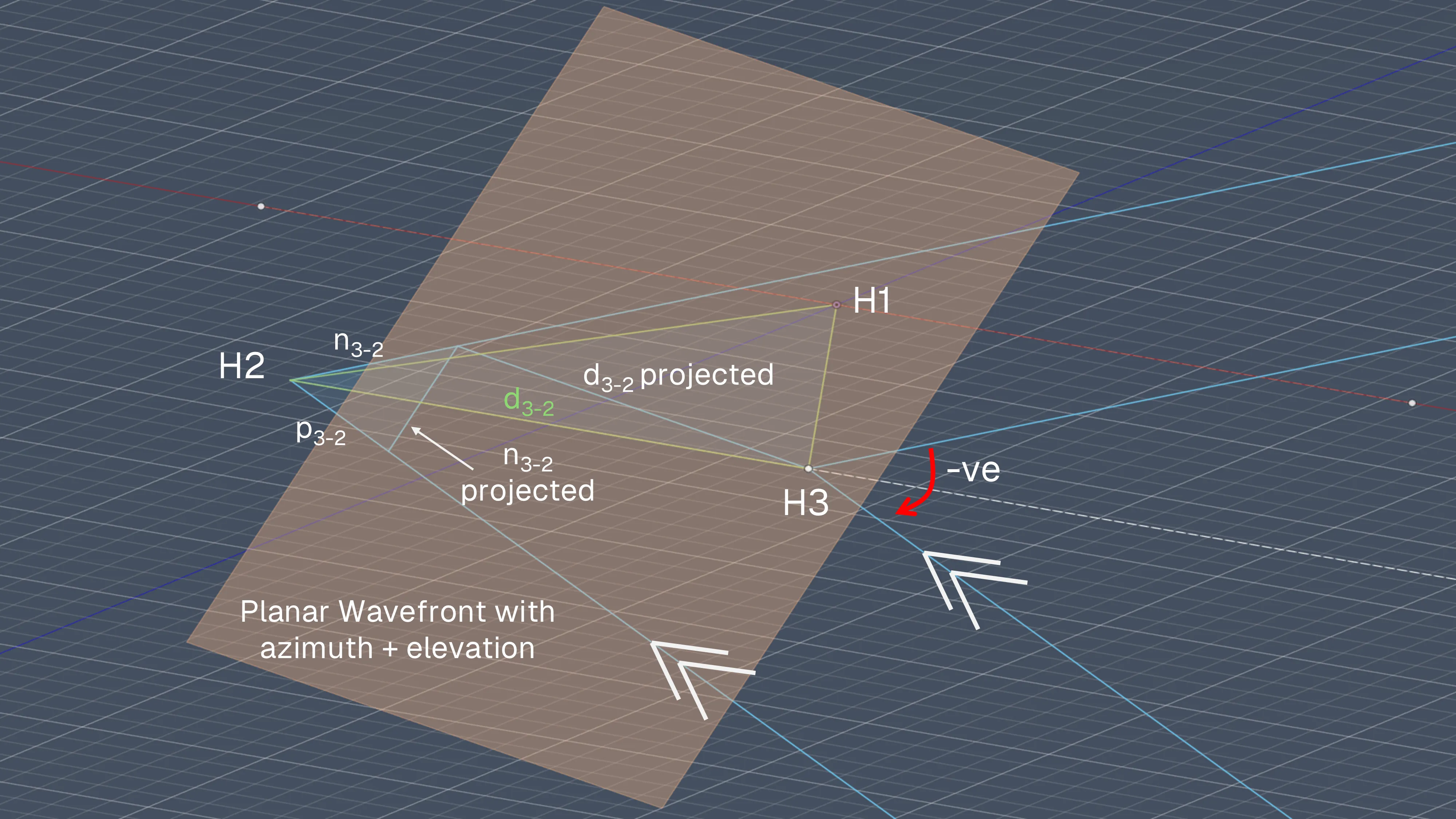
Assuming a far-field model (i.e. planar wavefront, not spherical), I first looked at the azimuth angle only. Looking at the line between H3 and H2, , and the projection of this line onto the planar wavefront, it can be seen that the normal vector between both lines yields the path difference between hydrophones 3 and 2, labelled . Then, adding in the elevation angle, the normal vector between and its projection onto the new wavefront yields the actual path difference for the signal denoted as .
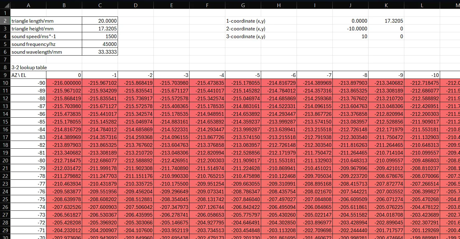
Before immediately diving into more math/code, I wanted to visualise this problem on Excel first. Hence, I aimed to create a table of all the expected phase differences given every possible azimuth and elevation angle (in intervals of 1 degree). Deconstructing the triangles involved, I get the following equation to find each entry of the table:
where is the vector of azimuth angles ranging from -90 to 90 degrees, is the vector of elevation angles ranging from 0 to -90 degrees, is the distance between hydrophones, and is the pinger signal’s wavelength. The piecewise function helps with looping around for phase differences larger than while preserving the positive/negative sign to indicate which signal is leading/lagging.
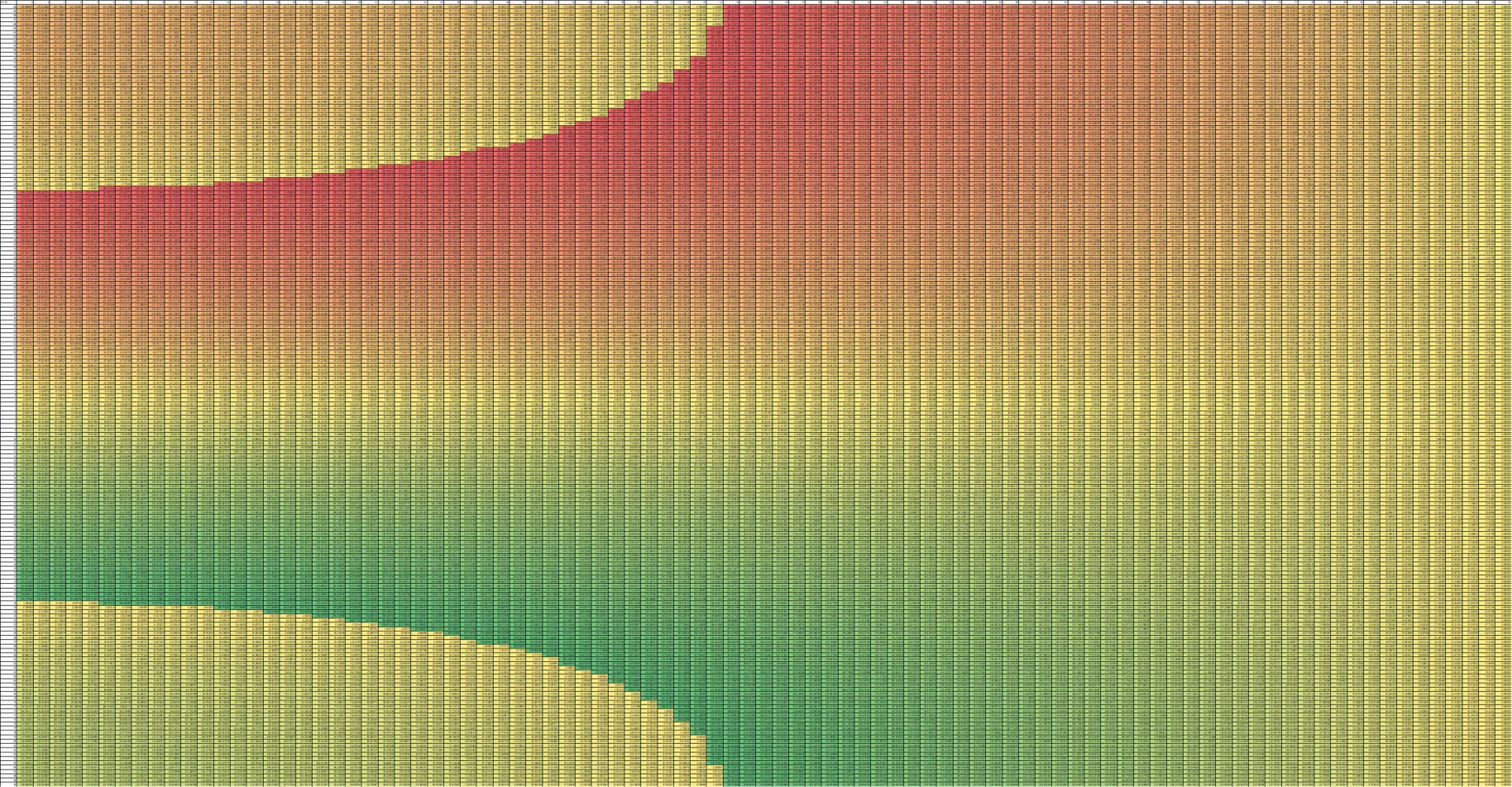
The tabulated data was coloured with a red-yellow-green scale for clarity. Redder regions indicated more negative numbers, yellow regions were close to 0, and greener regions indicated more positive numbers. The left image below shows a close-up of the table, where azimuth angles go along the rows (y-axis) and elevation angles go along the columns (x-axis). The full table on the right makes intuitive sense too. At the middle of the table where azimuth is 0, changes in elevation angle will still keep the phase difference at 0. At the right end of the table where elevation is near -90 degrees (i.e. the source is directly underneath the hydrophones), azimuth angles (rotations about Z axis) make minimal difference to the signal path, hence keeping the phase difference near 0.

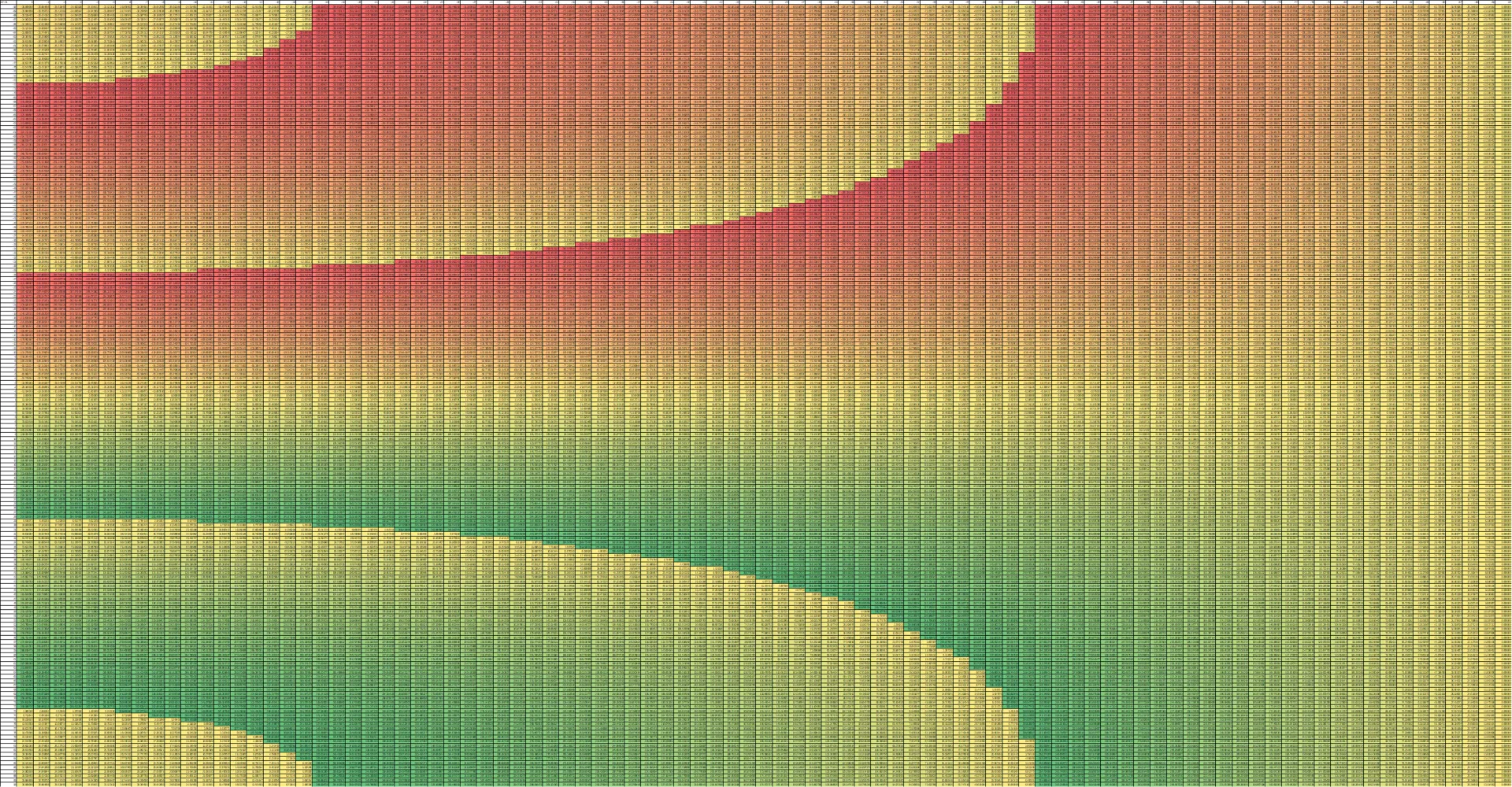
The aliasing issue also becomes visually obvious in this table by varying the hydrophone spacing . When like in the table above, there is no aliasing, i.e. every azimuth-elevation pair corresponds to a unique phase difference value.
However, when (the actual final spacing used), the phase differences loop back around to 0, which are shown by the border where colour changes abruptly in the left image. When , the phase difference loop back around twice, hence the “double border” in the right image.
Note: Literature regarding grating lobes will state that the spacing distance should be below to avoid aliasing, which is true if purely relying on phase differences since it becomes more ambiguous which is the leading/lagging signal for phase shifts beyond or .
However, as I am still able to differentiate the order in which the hydrophones received the signal (just not at a high enough accuracy to do TDOA), I can recognise the leading/lagging signals all the way up to one phase shift (). Hence, my spacing distance to avoid aliasing can go up to .
To create the simultaneous equations needed to solve for azimuth and elevation, two pairs of phase differences are needed. The other pair I used was the phase difference between H3 and H1. The same formula could be used except the azimuth angle had to be shifted by .
Rewriting the equations to solve for azimuth and elevation by dividing ,
where were integers with range . The function of is to account for all possible positions due to the aliasing (i.e. the result of “inverting” the mod function) and its range is only because the aliasing only occurs up to one extra wavelength.
For the actual algorithm, all 25 possible azimuth angles are first calculated by varying . Thereafter, the elevation angle is calculated using the respective azimuth angles. If the azimuth-elevation angle pair is not possible for a given , the fraction within the function will exceed a magnitude of 1, and thus have no solution. Hence, as long as a solution exists for the elevation angle, then the azimuth-elevation pair of angles are considered possible solutions.
Once all the possible azimuth-elevation pairs are found, based on the coarse order of when each signal arrived at each hydrophone, the signal must have come from one of the six 60 degree wedges, as shown in the diagram below. For instance, if the signal is between 0 to 60 degrees the ping would be first detected by H1, followed by H3, then H2.
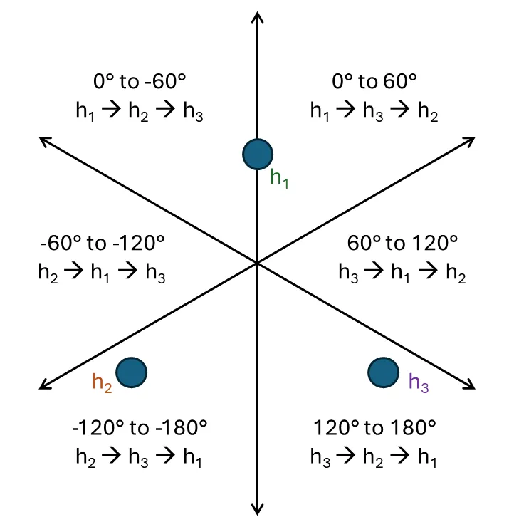
This is sometimes enough to resolve to a single pair of azimuth and elevation angles, but for the remaining cases, it was planned to fuse with camera data (which could tell where the buckets were located), to get a better estimate of where the pinger should be. However, the temporary fix for testing purposes was to just use the vector closest to the last calculated vector using cosine similarity.
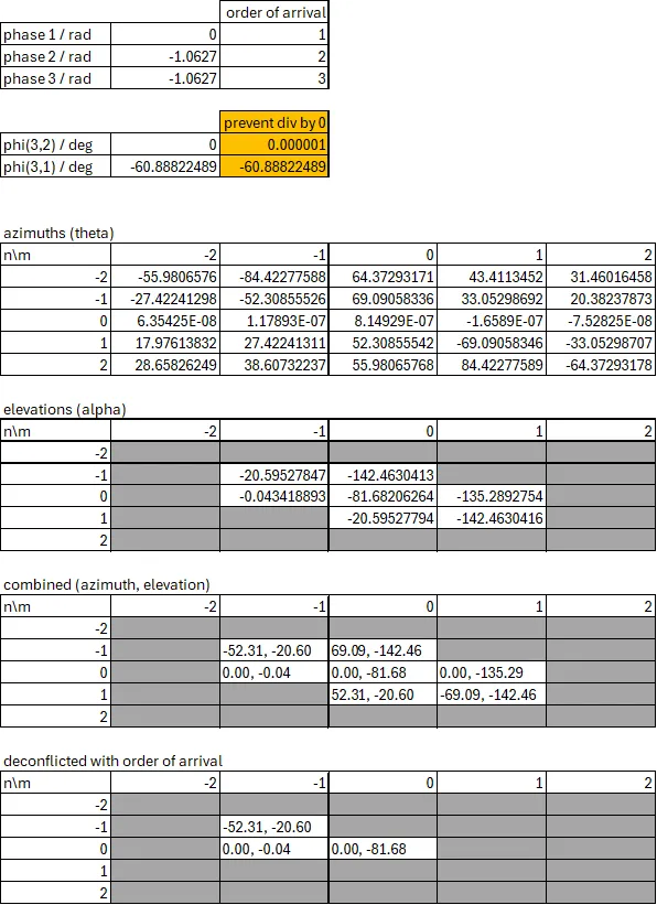
A sample example using Excel is shown below. If the source was directly in front of the hydrophone array (i.e. azimuth and elevation at 0 deg), then the expected phase difference between H1 and either H2/H3 is: . Using these phase inputs as well as indicating the order that the hydrophones would detect the signal in, yields 3 possible locations, one of which being the expected azimuth and elevation.
Results
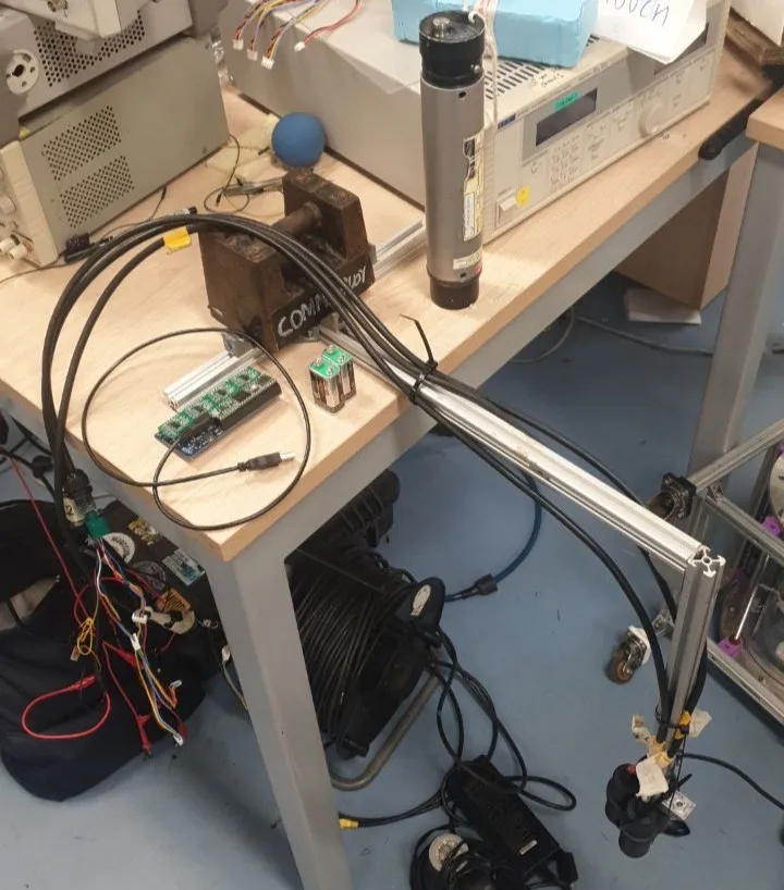
Due to other issues with the AUV, there was insufficient time to incorporate the acoustic system into the AUV for the competition.
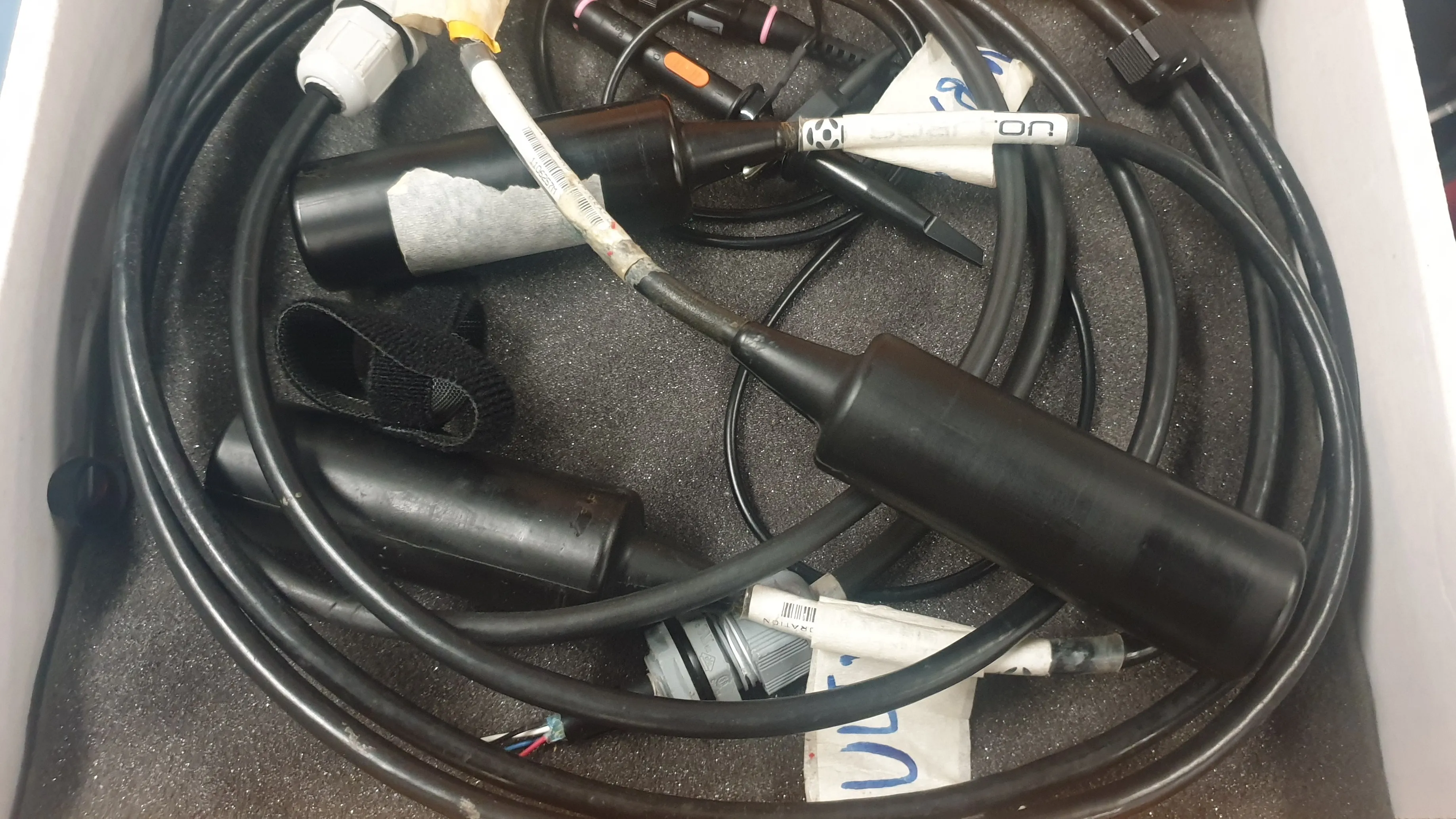
Luckily, data had been collected in the pool prior using the testing rig shown below. To ensure the collected readings were accurate to what the actual algorithm used, the readings were stored into the Teensy’s RAM2 which is optimised for access by DMA, thus ensuring the CPU is not occupied when datalogging. The entire datalog was also written to the SD card only after the ping was over.
Data for the following cases were collected:
- Azimuth: , Elevation: (on the left, near)
- Azimuth: , Elevation: (in front, near)
- Azimuth: , Elevation: (on the right, far)
- Azimuth: , Elevation: (directly underneath, near)
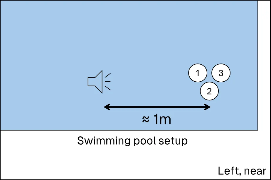
Feeding these collected data points into the algorithm yielded results that roughly matched the angles during setup. The images below depict the results from the first case.
- The first image on the left shows the pool setup where the pinger was placed about a metre away from the hydrophones and resting near the bottom of the pool.
- The next image in the middle shows the collected data, graphed using Desmos.
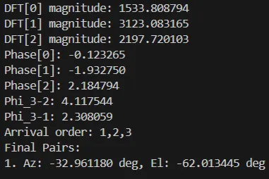
- The last image on the right shows the printed output from the Teensy after manually writing the collected data into its buffer arrays. Note that the calculated azimuth is around -30 degrees, which is correct since the final arrangement is rotated 60 degrees clockwise compared to the arrangement used in the pool.
While it was unfortunate that the system was not implemented in the final vehicle, the accurate results from actual data allows me to be confident that it would have worked effectively in the real world.
AUV’s Overall Architecture
When overseeing the design of the electrical architecture of the AUV, my main concern was with the overall maintainability of the system. From my internship experience in BeeX earlier in 2024, as well as looking at the AUV designed by the previous Hornet batch, the hull-based design for AUVs required proper planning for cable management, which is something that many newcomers can easily overlook.
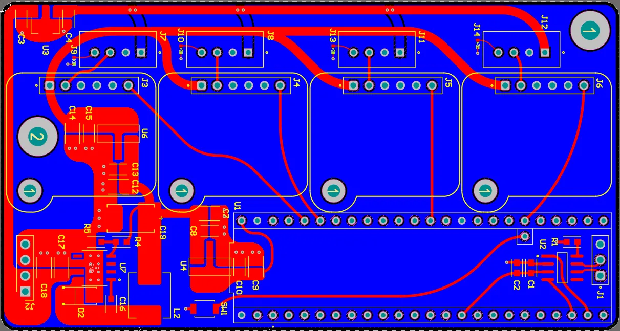
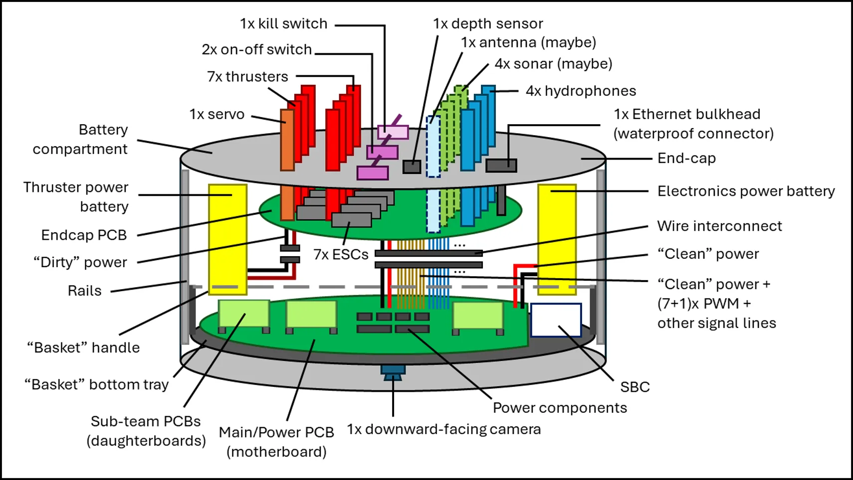
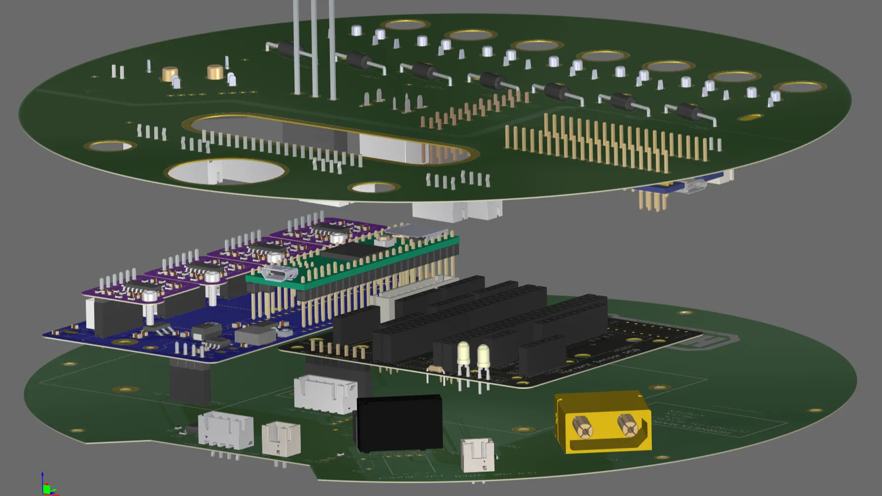
The initial draft for the electronics stack, as well as the final PCB multi-board assembly is shown below.
For connections to external devices, ideally, underwater connectors should be used. This is so that when the hull had to be opened, the external connectors could be unplugged and the hull cover can be removed fully. However, those connectors are expensive, and thus the cheaper alternative, cable penetrators/glands, were used. These were essentially rubber seals that compressed around a wire that fed directly into the faceplate.
These external wires connected to a faceplate (or “endcap”) PCB. This PCB contained all the electronics for actuator control and power switches. It also acted as a “pass-through” junction for external sensors, where wires from multiple sensors are re-routed to a single large connector. Noisy power used for the thrusters are also isolated from the cleaner power used for the internal electronics.
Wire management for the internal electronics was also kept neat by simply minimising the use of wires in the first place! A stacked design was adopted so that no wires were needed for inter-board communication. Connections between the external devices/endcap PCB to the main board stack-up, were bundled into 2x 20P Molex Micro-Fit interconnects. Hence, when removing the faceplate, only those 2 connectors, the battery and the Ethernet port had to be unplugged, which was a significant improvement from prior Hornet AUVs where there were individual wires that connected directly to the base boards.
Conclusion
On a personal level, this initial foray into acoustics systems exposed me to the world of analog electronics and signal processing, which was definitely an eye-opening experience.
While an ungodly amount of time was wasted spent staring at a whiteboard completely stumped, I was able to genuinely learn new things.
“Type-2 fun” as some might call it.
On a team level (within the electrical team), while it was quite a big group of 17 members, the overall process felt quite smooth sailing and I believe everyone had a chance to contribute and learn even if they were not planning to continue into the Bumblebee main team. I would generally attribute this to having a clear architecture defined from the start with a healthy number of motivated people, allowing for deadlines to be met largely on time with very few major faults happening during the testing phase.
On the Hornet programme level however, and even with the Bumblebee main team as a whole, the best word I could find to describe the overall vibe was… corporate. This is by no means saying it is bad; with a storied history of 10+ years and a really large team of 40+ members at any one time, it is essentially necessary to have a clear organisational structure and explicit division of labour to ensure deadlines and roadmaps are adhered to. It is also thus expected for such a structure to seep its way into how the Hornet programme was run.
Nonetheless, contrasting this with the hodgepodge 3/4-man team that was my years of RoboCupJunior experience, there did seem to be a dilution of that blend of domains that made robotics special; a regretful loss of interdisciplinarity is how I would phrase it. The split between the mechanical, electrical and software teams was quite stark, which resulted in a non-trivial amount of issues arising from integration hell. The large team size also meant that in order to split the work evenly, the assigned responsibility per person was rather small (or at least started out small). This meant that there was a limited sense of ownership, which resulted in both quality and general interest levels to take a hit. At least that’s just my read on things.
I wish there was a way to know you’re in the good old days before you’ve actually left them.
~ Andy Bernard (The Office)
← Back to projects